


Fatigue failure analysis combines engineering and science: science is attempting to tell us why the fatigue failures happen, while engineering must predict when failure will happen. Any machine, including components of any tramway installation, must be designed and manufactured with a reliability that will ensure a long and trouble-free life, and at the same time produce profits for the operator.
It is surprising how little is generally understood about the actual mechanisms of metal fatigue. Science has not yet completely explained it. The existence of the most talked about “endurance limit” of the material has been assumed, but never proven. Yet it has been said that 90 percent of all service failures are caused by fatigue, and that 90 percent of all fatigue failures are caused by improper design.
This statement could not be more true when applied to the components of aerial tramways. Barely an operational season goes by without chairs developing fatigue cracks, and in extreme cases, bullwheel shaft failing.
Since the science is not available, the engineers must design the parts based on whatever knowledge is available. Most fatigue failure knowledge is statistical in nature. Using an analytical approach, one can achieve fairly meaningful results in designing the part for infinite fatigue life or predict when the failure will occur in the case of finite life expectancy.
Fatigue Failure Described
Since there are numerous fatigue failures occurring constantly on tramway installations, any person involved in the subject is familiar with the appearance of the failed part cross-section.
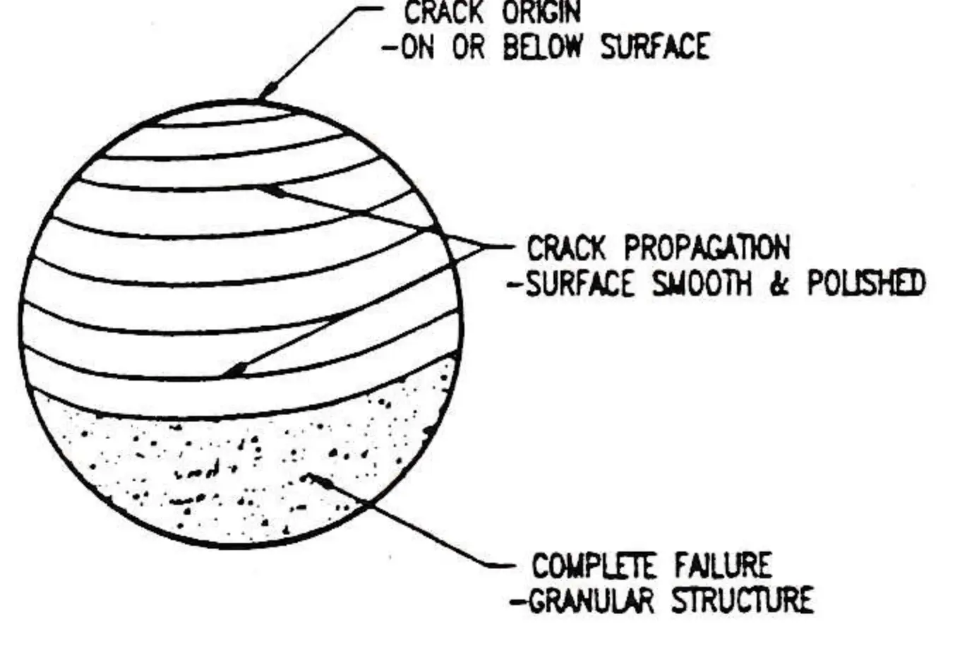
The Fig. 1 graphically describes the typical fatigue failure of a round shaft. The failure always has its origin in some surface or below surface material imperfections or discontinuities. They are described in the details later in the section on factors that modify endurance limit.
The failure begins with the development of a small surface crack which, under subsequent alternating loads, continually opens and closes. This movement causes the adjacent surfaces to rub against each other making both surfaces smooth and polished in appearance. This process, called crack propagation, can last quite a long time depending on the magnitude of the load and properties of the material.
Finally, the remaining area of the cross section is not big enough to withstand the load and the break occurs suddenly. This final cross section area has a granular structure and almost resembles the brittle, static failure. The two different regions in a fatigue fracture are very useful in analysis of the part failure.
Statistical and Analytical Approach
In designing the part against fatigue failure we start with the available information describing the basic properties of the material. (Reference will be made only to the ones used in this analysis, even though there is much more available.) One of the first problems in fatigue design is to find the general relationship between the fatigue properties of the material and the strength obtained from a simple tension test.
As a reminder let’s review the basic properties of the material in very simplified form. Tensile strength, also called ultimate strength (Sut), is measured in pounds-per-square-inch and represents the highest stress that material can sustain during the tensile test. Strain in the tensile testing, measured in inches-per-inch, is defined as the change of the specimen length divided by the original gauge length, so it can also be expressed as percent of elongation. After the specimen is subjected to the tensile test, the results can be plotted on x-y axis using corresponding stress values versus percent of elongation. See Fig. 2.
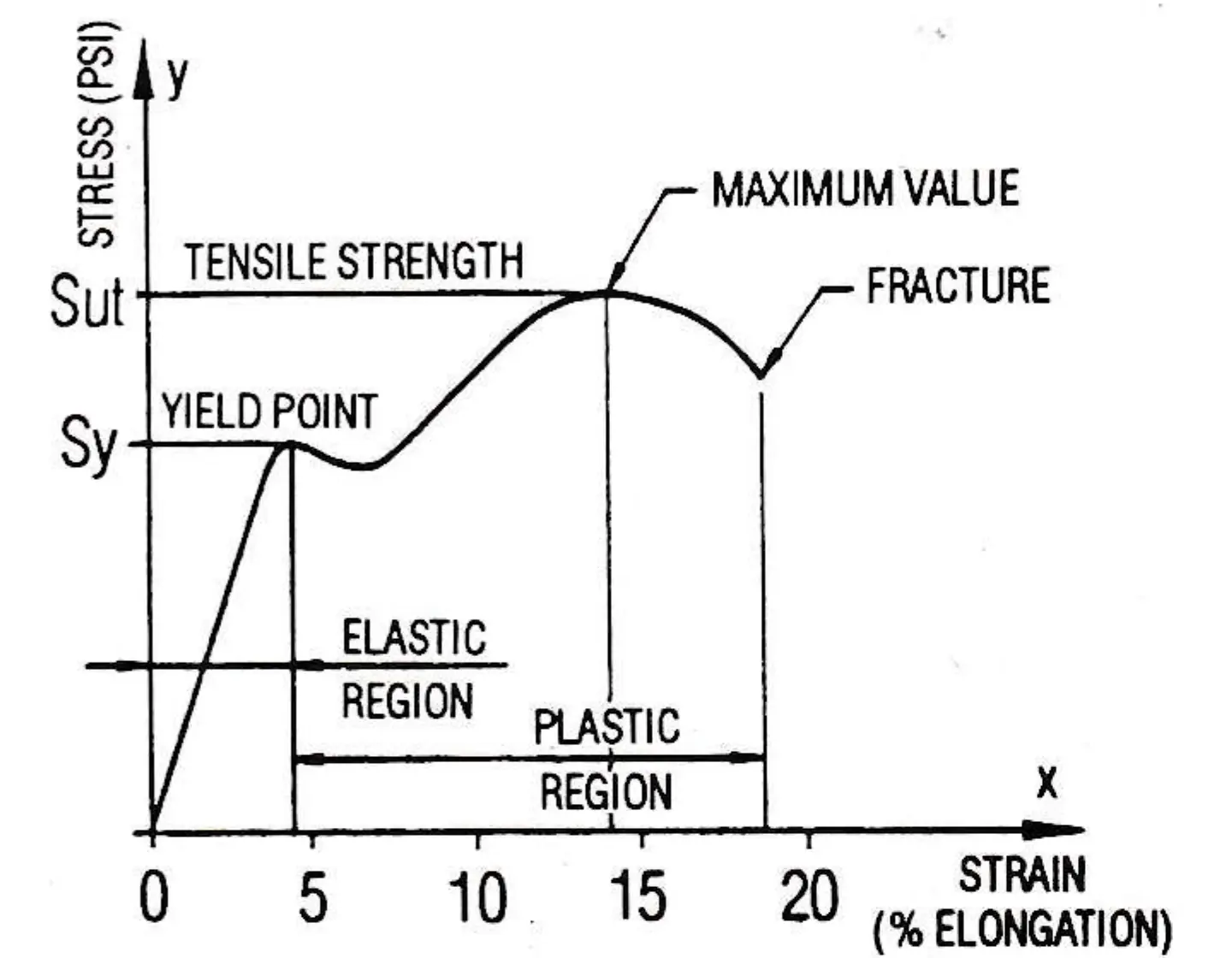
Up to the yield point stress (Sy), the material behaves in an elastic manner; that is, it will return to its original configuration when the load is removed. Above the yield point the material starts stretching permanently, while still maintaining the load. This is referred to as the plastic region.
After reaching the tensile strength stress, the specimen fractures at a somewhat lower stress, called fracture strength. The stress-strain curve is different for each type of material, depending on the properties.
The tensile test is a static type of test. When it comes to fatigue we have to add two more variables: fluctuating stress and time expressed in cycles. For this we need another type of test which can determine the strength of the material under the action of fatigue loads.
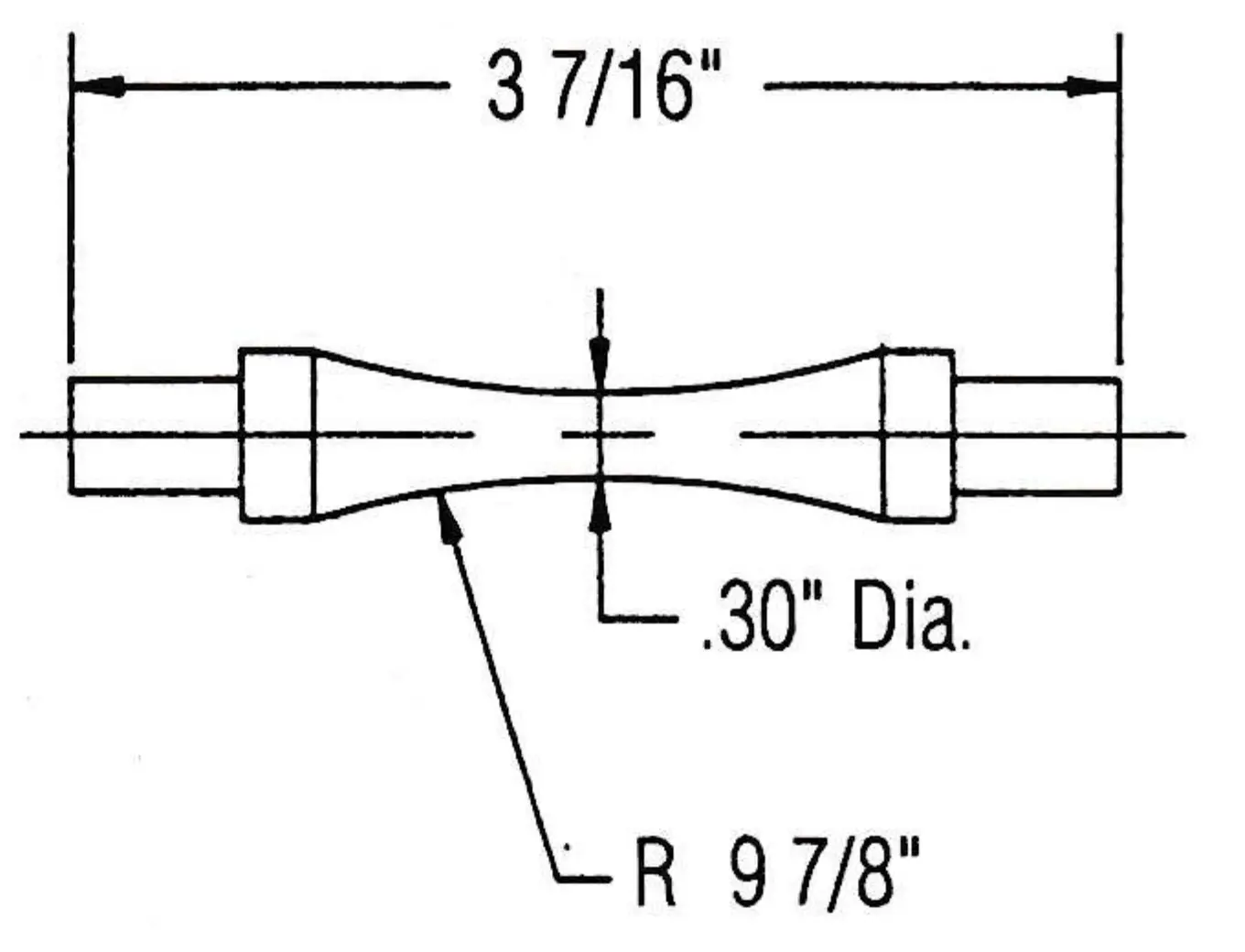
The most widely used device for this type of testing is the R.R. Moore high-speed rotating machine. It uses specimens shown in Fig. 3 which are subjected to varying loads of known values; the cycles or stress reversals are counted to destruction.
It should be noted for future reference that the specimens used for fatigue testing are very carefully machined and polished in both radial and axial directions. The ultimate goal is a test specimen with no surface imperfections.
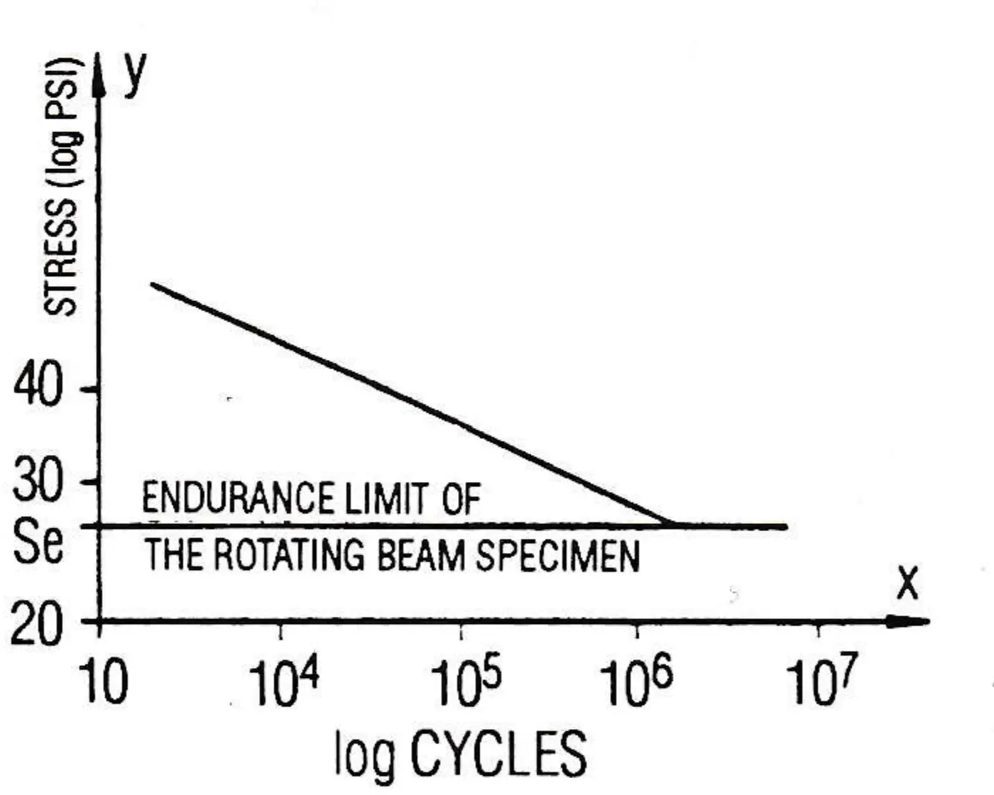
Because of the statistical nature of the fatigue, quite a number of tests are necessary to establish the fatigue strength of a particular material. During the rotating beam test, the first test is made at a stress level just below the ultimate strength of the material. The number of cycles is recorded at specimen failure. The next test is made with lower stress than the previous one, and the process is repeated until the stress reaches a value at which the specimen failure will not occur, no matter how great the number of cycles. This minimum stress is called endurance or fatigue limit (S’e). The results of the above tests are shown in Fig. 4 and the corresponding diagram is called S-N diagram.
This diagram applies only to ferrous materials. In the case of aluminium the curve never becomes horizontal, since non-ferrous materials do not have endurance limits. In their case the fatigue strength must be specified with corresponding cycles the material endured before failure.
When all available data from tension and rotating beam tests were analyzed it was found that there is a relation between the results of these two tests.
All of the above data and consequent conclusions are of a statistical nature. Even if they are imperfect, they allow an engineer to start designing the parts for fatigue failure by using the following equations where S’e stands for endurance limit and Sf for fatigue strength:
- S’e = (0.4 to 0.6) Sut for steels with tensile strength below 200,000 PSI.
- Sf = (0.16 to 0.38) Sut for aluminium allows based on 500 million cycles and depending on the manufacturing process and tensile strength.
Designing the Actual Part
Having established the endurance limit of the rotating beam specimen, one can now start designing the part itself which of course, differs from the “ideal” rotating beam specimens. It may be of different size and shape, and a large number of other variables enter the picture: it may have been manufactured using different methods; it may have been exposed to heat treatment; it could have been welded or assembled under force. Perhaps it has a sharp corner, perhaps its surface was treated, perhaps it is to work in the hostile outside environment. The actual part will also be exposed to different types of loads, some of a very complex nature.
The end effect is that the original endurance limit S’e must be corrected, taking into account these modifying factors, to arrive at the actual part endurance limit Se.
Following are the most important factors modifying endurance limit:

Surface finish – ka – For highly polished surface rotating beam specimen ka=1. It becomes smaller for parts which are ground, machined cold or hot rolled, cast or forged. Depending on the tensile strength of the material, the surface finish factor can drop top as low as 0.2.
Size effects – kb – The rotating beam specimen is 0.3 inch in diameter. It was found that endurance limit of larger parts can be up to 25% less. It is accounted for by the fact that large parts will have more surface imperfections.
Reliability – kc – This factor includes the material variation in evaluating the mechanical component. Most plots and tabulated data of endurance values are mean values. If used as such they will yield 50% survival rate. The correction for different reliability levels assumes 8% of the endurance limit standard deviation, provided the material used conforms to minimum values of strength properties.
- kc= 1 for 50% reliability
- kc = 0.814 for 99% reliability
- kc = 0.702 for 99.9% reliability
Temperature effects – kd – This factor does not affect the lift components since these are not exposed to temperatures above 160° F. The low temperatures actually increase the endurance limit of carbon and alloy steels. The low temperature consideration should be given to elastomer and rubber parts.
Stress concentration – ke – This is one of the most important modifiers of the endurance limit. In using the basic static stress equations it is assumed that the cross sections involved are constant with no irregularities and imperfections, whereas in real life mechanical parts have all kinds of imperfections and discontinuities present, such as holes, grooves, keyways, notches, abrupt changes of diameter and sharp radius’s. Any of these imperfections change the stress distribution by raising the local stresses up to three times.
Stress concentration effect exists in a very small region of the discontinuity. When the first load is applied, the high stresses cause the yielding of the discontinuity, which in effect relieves the stress concentration. This is a normal occurrence for static loads. What happens is the remaining structure takes over and the part is as strong as the intended design.
Unfortunately, if the load continues to fluctuate, the stress concentration area becomes the origin of the fatigue crack and has catastrophic consequences. There is a lot of information available for proper selection of the concentration factors, and in connection with material notch sensitivity one can accurately calculate the endurance limit modifying factor. The values of ke in the extreme case can be as low as 0.3.
Miscellaneous effects – kf – There are countless other factors affecting the endurance limit. Some of them can actually increase it by building the compressive stresses into the surface. Cold rolling and shot peening belong in this group.
Among the factors which reduce the endurance limit are corrosion, metallic coatings such as chromium, nickel, cadmium and zinc plating, welding, galling, abrasion, pitting and fretting caused by minute movements between mating surfaces, as in press fits.
By multiplying the original specimen endurance limit (S’e) by all the applicable modifying factors (k) one can arrive at the endurance limit of the actual part (Se) which can be used in further calculations.
It is common to start with 150,000 PSI tensile strength materials and end up with an endurance limit in the 10,000 to 20,000 PSI range.
Fatigue Strength Under Fluctuating Stresses
Having established the endurance limit we can now evaluate how the applied loads will affect the fatigue life of the part. The fatigue stress is the fluctuating stress which can alternate between tension and compression or between certain steady level of stress initially imposed on the part. The basic type of fatigue stress is shown in Fig. 5.
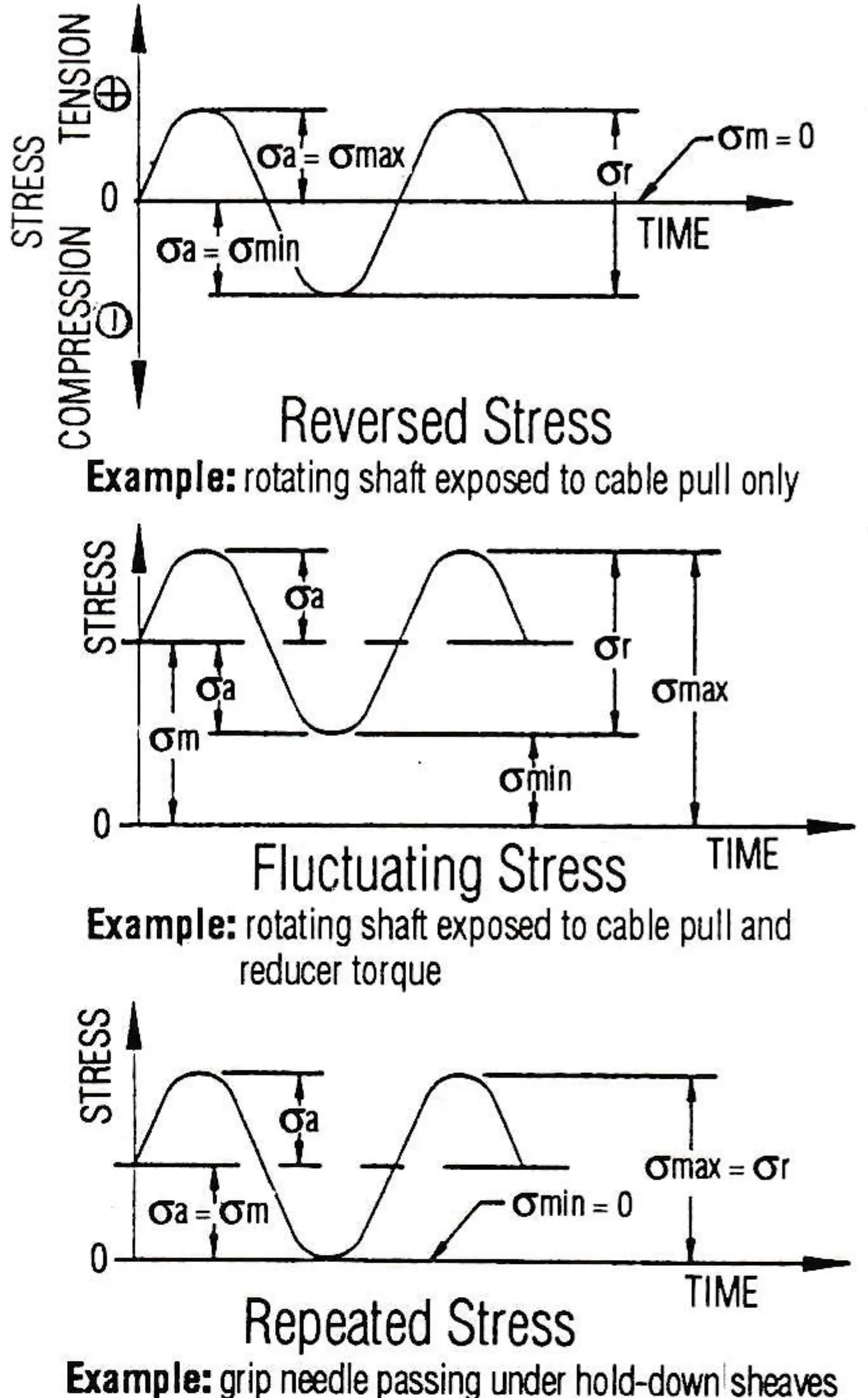
It is most important to establish the maximum and minimum stress when designing or analyzing the part for fatigue life. These can be either calculated, measured during the actual load conditions using the strain gauge technique. The latter method requires building a prototype, or several of them, and is of course mush more expensive. It is also the most accurate. the stresses involved may be of a simple kind or much more complex, involving combinations of several types.
Having the stresses established, we can plot them on a fatigue diagram, for which there are three to choose from: Soderberg’s, Goodman’s and Gerber’s. Soderberg and Goodman are very similar but the Soderberg is used here because of its simplicity to understand and because it is the most conservative (Fig. 6 and caption).
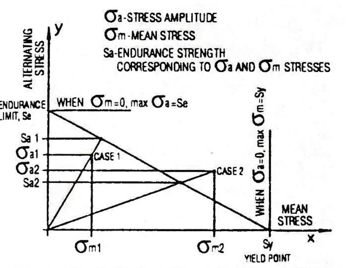
From everyday observations at different ski areas we see parts and components of the tramway installations falling after a certain time in operation. In all those cases the combination of fluctuating and mean stresses fall above the Soderberg’s line and the safety factor is below one. The life of the part in such a case can be calculated in terms of cycles to destruction by using additional statistical and analytical information (see Figure 7 and caption).
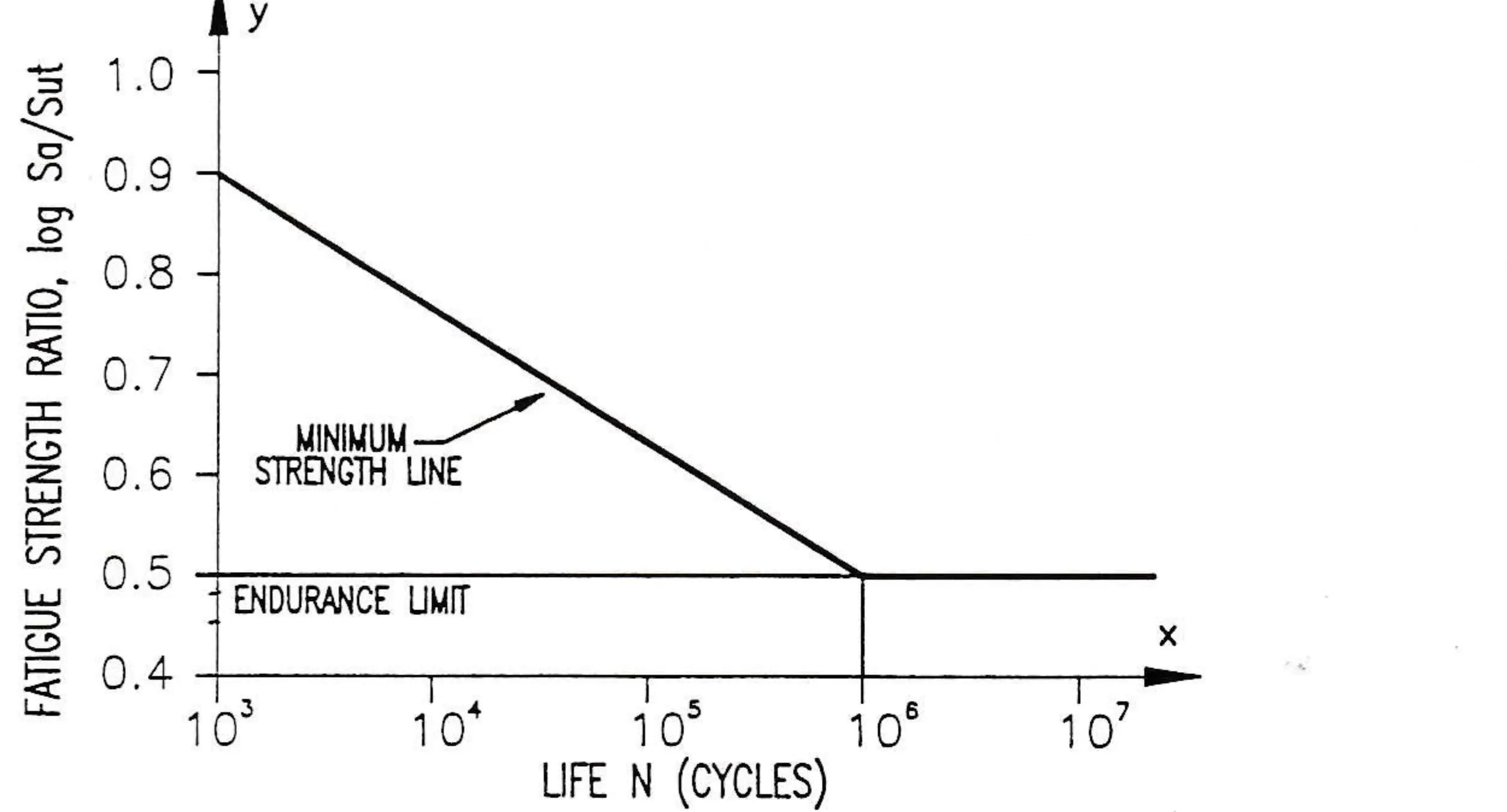 Fig. 7 – The relation between the fatigue strength ratio and the life of the part. From the results of a very large number of fatigue tests on various materials and strengths, a plot of fatigue to tensile strength (Se/Sut) was obtained. The curve shown represents the minimum strength line as the one recommended to be used in calculations. One point of this line corresponds to Se/Sut = 0.9 at one thousand cycles, and the other to endurance limit Se at one million cycles. The line can be then expressed as the following equation: log Sa = -m log N + b to define the mean fatigue strength. Sa corresponding to any life N. where: m = 1/3 log (0.9 Sut / Se) and b = log ((0.9 Sut)2 / Se). The equation can be then solved for life of the part exposed to any stress amplitude: N = 10b/m / Sa1/m (cycles), 103 ≤ N ≤ 106.
The fatigue failure and its catastrophic consequences can be predicted and prevented. The best prevention is proper design. Sometimes it may require intensive and costly testing.
The second approach is to take advantage of the crack propagation phenomenon. It happens in the plastic region of the material behavior, but it takes time before it leads to complete failure. This time allows us to catch it and prevent it from further spreading. Proper inspections are of utmost importance in this case. Analysis and calculation of the time to failure will help to program the proper intervals for these inspections.