


Columnist Richard D. McHugh is president of Skier Feeding Inc., a food-service consulting firm specializing in ski area feeding. He is the hotel and resort management department head of the Washington County Vocational Technical School in Calais, Me., and was general manager of food and beverage concessions at Mt. Snow, Vt., for A.B.C. Consolidated, a subsidiary of Ogden Foods. He is a graduate of the Hotel and Restaurant Management School at the University of Massachusetts.
Plotting today for tomorrow
Few readers will argue against the point that record keeping is a bore. At the same time, there are very few administrators who would not welcome more precise data when decisions must be made. In any field, it still seems that a prerequisite for knowing where one will be tomorrow is knowing where one is today.
Perhaps the quickest way for getting a handle on any operation is a daily tally sheet. It will not tell the internal rate of return, the gross fixed asset turnover or the recommended discount rate to use for present value calculations, but it will show how many people came to your area, how much they spent and where they spent it. As with any fill-in-the-blank game, the tally sheet can be as simple or as complicated as the designer wants to make it. Keep in mind, however, that your girl-Friday will more likely keep it up to date if it is simple.
The tally sheet shown in Fig. 1 does not concern itself with product cost, or any cost for that matter. It only involves itself with revenues and numbers, the important numbers being skier days and employee days. For evaluating performance or making projections, the tally-sheet data provides a measure of departmental demand as well as the amount of human capital apparently necessary to support that demand.
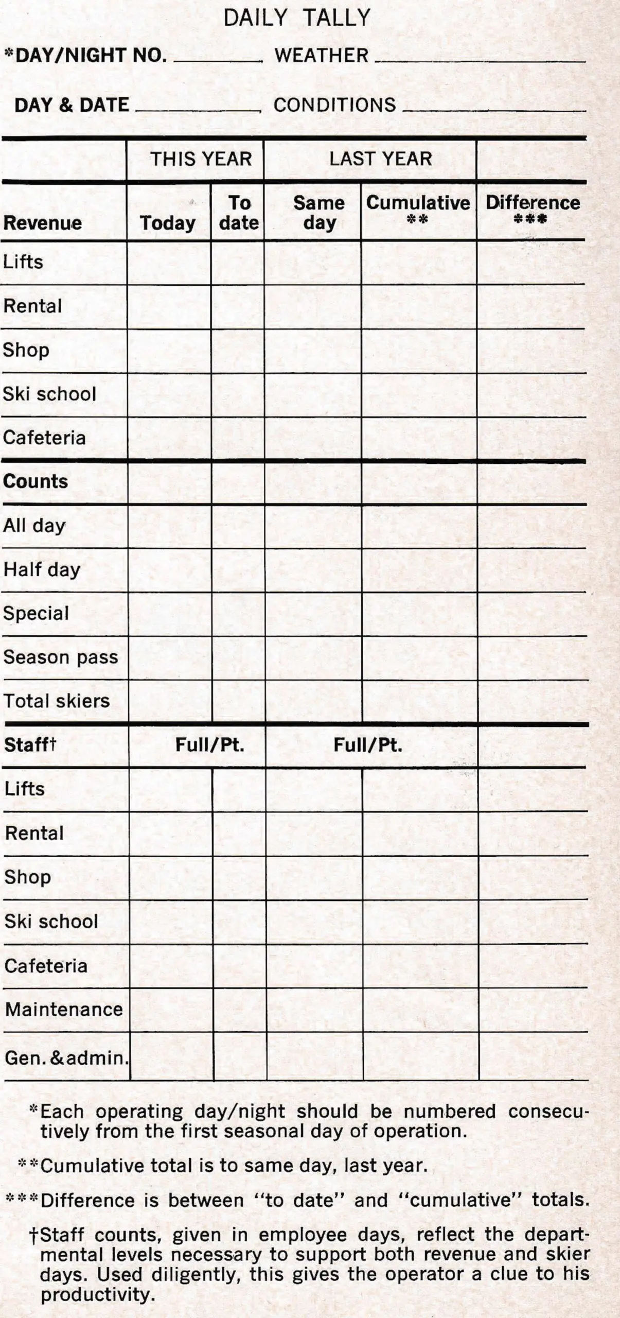
To illustrate the practicality of a simple tally seet, consider operator A, B and C, who have identical operations and had exactly the same revenues and numbers of skiers last year. All are trying to determine the probable performance of their cafeteria next season.
Operator A reasons simply that the $75,000 in cafeteria revenue is equivalent to 18.75 per cent of his $400,000 lift revenue and since his lift revenue is 15 per cent higher than the previous year, he will likely do $460,000 (reflecting another projected 15 per cent increase in lift revenue next year) x 18.75 per cent or $86,250 in cafeteria revenue next season.
Operator B sets about more ambitious forecasting and prepares a five-year regression analysis of cafeteria sales, taking care to adjust for year-end price changes which had a differential greater than one standard deviation when equated to constant dollars using the old 1958 consumer price index. The resultant annual compound growth rate was then further corrected for the recent rise in Aaa bonds while common stocks on the Big Board were falling, thus indicating a possible tapering in vacations by the carriage trade. Since sales potential is a function of capital investment, Operator B concludes that multiplying his growth rate by initial cafeteria investment from which diverted funds had been deducted and then factoring this by the turnover rate, he would derive the approximate volume for next season. Thus:
[g( I − Σfd)] T = Volume

Based on these calculations, operator B predicts his cafeteria revenues will increase from $75,000 to $84,375.
Operator C, on the other hand, uses an approach less involved than B’s but somewhat more accurate than A’s. He has experienced growth comparable to other areas in his state over the last several years and available data indicates that skier days are currently increasing at approximately 12 per cent a year. C is putting in additional snowmaking equipment this summer and is confident that it will add 15 days to his 100-day average.
To begin with, Operator C has, as is shown in the table at right, totaled the columns in his tally book and then broken down the cafeteria amounts between week days and weekends for each month. First, by dividing the respective total skier days each month into the appropriate revenues, he can determine last season’s per-skier spending in his cafeteria.
| Total Sales | December | January | February | March | April |
|---|---|---|---|---|---|
| midweek | $5,040 | $3,190 | $9,880 | $9.200 | $420 |
| weekends | $3,600 | $13,600 | $13,300 | $13,680 | $3,060 |
| Total Skiers | |||||
| midweek | 5,600 | 4,250 | 12,350 | 11,500 | 600 |
| weekends | 3,600 | 16,000 | 14,000 | 15,200 | 3,600 |
| Average Skiers | |||||
| midweek | 800 | 250 | 650 | 500 | 150 |
| weekends | 1,800 | 1,600 | 2,000 | 1,900 | 1,200 |
His experience tells him that 80 per cent of the 12 per cent growth in skier days will be felt on weekends, and he expects to get his 115-day season off the ground next December 17, with no major changes in the cafeteria. All the operator need do is, using a calendar, break down his upcoming season into midweek and weekend days for each month throughout the season. Applying projected growth rate to last year’s average skier days and using the same spending patterns, he arrives at a projected revenue figure of $93,214, representing a 24 per cent increase.
Cafeteria projections are, of course only one of the tally-sheet possibilities in predicting your season’s sales. Operator C’s model, as outlined here, can be used in forecasting revenues for virtually any department.